10. Wave modeling¶

An important application of the ComFLOW program is the simulation of wave impact on offshore structures. ComFLOW provides various built-in wave models as well as the possibility to import custom data by means of plug-ins. By means of plug-ins and coupling to other software it is possible to simulate a wide range of other wave conditions (e.g. irregular waves). The wave models can be used for initialization or as input for boundary conditions.

10.1. Built-in wave models¶

The wave model can be selected by setting the key waves/model/@model to any of the available built-in models (or set it to "none" if no wave model is required).

10.1.1. Common attributes¶

The built-in wave models have the following attributes in common:

`waves/@mean_depth`	The mean water depth in meters. If the water depth is set to zero it is determined at run time and is set equal to `-zmin`. The same holds when no incoming wave is specified, that is, when `waves/model/@model="none"`. Note that the mean depth is used in various parts of the program, for example in the absorbing boundary conditions.
`waves/model/@dispersion_mode`	This attribute can be set to `"calculate_k"` or `"calculate_omega"`. By default this attribute is set to `"calculate_k"`, which means that the wave properties are determined by the wave period (`@period`) and the dispersion relation is \(\kappa(\omega)\) used to calculate the wave length. If set to `"calculate_omega"`, the wave properties are determined by the wave length (`@length`) and the dispersion relation \(\omega(\kappa)\) is used to calculate the wave period.
`waves/model/@period`	The wave period in seconds.
`waves/model/@length`	The wave length in meters.
`waves/model/@height`	The wave height in meters (two times the wave amplitude).
`waves/model/@location_of_crest`	This attribute defines the location of the wave crest in meters at t=0.
`waves/model/@angle`	The angle of incidence of the wave, expressed in degrees with respect to the positive X axis.

10.1.2. Airy wave theory¶

The Airy wave model is selected by setting @model="Airy". The wave elevation is defined by a cosine: \(\eta(x,t) = A\cos(\omega t-\kappa x+\phi)\) with \(A\) the amplitude, \(\omega\) the frequency, \(\kappa\) the wave number and \(\phi\) the phase.

10.1.3. Linear irregular waves (plug-in)¶

Irregular waves by means of linear wave superposition.

10.1.4. Stokes wave theory¶

ComFLOW provides the second-order and fifth-order Stokes wave models. These models are selected by setting @model="Stokes-2" or @model="Stokes-5".

10.1.5. Rienecker-Fenton wave theory¶

The Rienecker-Fenton wave model is selected by setting @model="Rienecker_Fenton". Rienecker-Fenton wave theory gives more accurate wave kinematics than 5th-order Stokes in shallow water and for very steep waves. The order (higher harmonics) of the solution can be chosen freely as long as @order is lower than or equal to 256 (the default setting is @order="10"). Please note that higher-order waves may not be represented accurately on relatively coarse meshes. One should also note that Newton iteration is used to solve the nonlinear equations at the construction of the waves. The iteration does not always converge. Convergence is almost guaranteed for “realistic” waves, but convergence behavior may depend on the desired order of the solution.

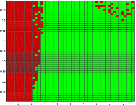
Fig. 10.1 Combinations of dimensionless wave height and wave period for which the Rienecker-Fenton solution converges (green) and diverges (red), when @order="10" and @mean_depth="10.0".

10.2. Background current¶

It is possible to specify a uniform background current in the XY-plane. Although it is possible to combine background current with any of the wave models provided by ComFLOW, the dispersion relation is only consistently modified when combined with Airy waves or Stokes-2 waves.

The current is expressed in terms of an angle (degrees) and a magnitude (m/s), which are defined by the attributes waves/current/@angle and waves/current/@magnitude, respectively.

10.3. Initial conditions and ramping functions¶

For smooth transition between different wave regimes it may be useful to ramp up or ramp down the amplitude of the wave(s). To accomplish this, various ramping functions are available in ComFLOW.

The initialization of the wave field at t=0 is controlled by the attribute waves/@start_with_still_water which can be set to "true" or "false". This variable must be set to "false" if a ramping function is used.

Ramping functions are enabled by setting the attribute waves/ramping/@ramptype to one of the available functions. the behavior of the ramping functions can be controlled with the attributes @ramp1 and @ramp2. A summary is given in the following table:

`@ramptype="0"`	no ramp
`@ramptype="1"`	linear upwards ramp to full amplitude during `@ramp1` wave periods
`@ramptype="2"`	linear upwards ramp to full amplitude during `@ramp1` wave periods, then constant for `@ramp2` minus `@ramp1` wave periods, then linear downwards ramp during `@ramp1` wave periods to zero amplitude
`@ramptype="3"`	undocumented

10.4. Guidelines for simulation setup¶

It is recommended to use higher-order discretization methods for convection and for the advection in the VOF method. Use grid stretching and local or adaptive grid refinement in order to efficiently obtain sufficient grid resolution around the free surface.