7. Setup of the computational grid
In this chapter, the local grid refinement module of ComFLOW is described in more detail. A part of the user input is described in Chapter 27. Guidelines will be given about how to set up a locally refined grid.
Note
If your simulation input contains the old-style input file comflow.in, make sure that the parameter griddef
in the grid input section is set to 2 (see fixed_form_input/computational_grid).
By means of the local grid refinement functionality of ComFLOW a grid can be locally refined or coarsened in order to obtain more accurate results or to save computational time. The starting point for local grid refinement/coarsening in ComFLOW is the so-called reference grid \(G_0\) at reference level \(\ell=0\). This can be any user-defined Cartesian grid, possibly with grid stretching (see Fig. 7.1). The building blocks for the computational grid now consist of \(G_0\) and its globally refined and coarsened counterparts \(\dots,G_{-1},G_{+1},\dots\) (these are the gray grids in Fig. 7.1). A computational grid is now obtained by selecting a domain-covering subset of the collection \(\{\dots,G_{-1},G_0,G_{+1} \}\). In Fig. 7.1 this is illustrated by the thick black lines.
Between each two subsequent refinement levels, the grid is coarsened or refined by refinement ratios \(r_i,r_j,r_k\), which are typically chosen uniform and equal to 2. However also other (anisotropic) combinations can be used, or directions can be excluded from refinement by setting the corresponding refinement ratio(s) to 1.
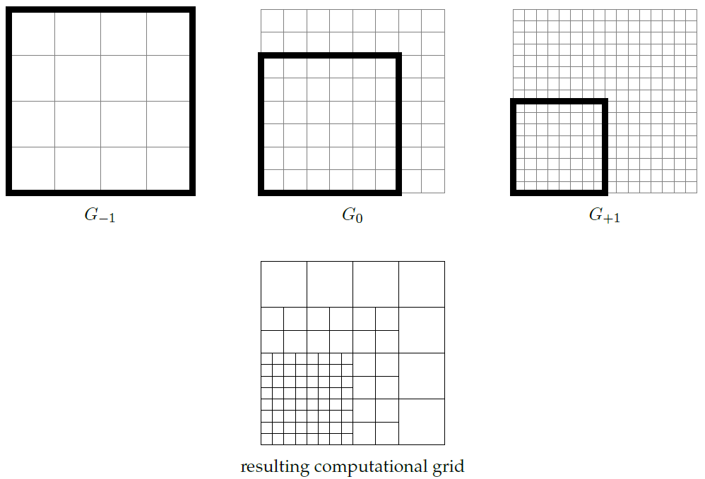
Fig. 7.1 Concept of the reference grid and local refinement / coarsening in ComFLOW. The Cartesian grid \(G_0\) at refinement level \(\ell=0\) (the gray grid in the middle) is the so-called reference grid as defined in the user input. The thick lines denote the actual (sub)grids that are used during the simulation.
7.1. Defining the Cartesian reference grid
The grid settings are specified inside the key /comflow/grid/. For details on how to use the XML input format consult Chapter 26.
Starting point for grid setup is the Cartesian reference grid at refinement level \(\ell=0\).
The dimensions of this grid are given by the parameters imax, jmax and kmax.
In order to run a 2-D simulation in the YZ (XZ) [XY]-plane set imax (jmax) [kmax] to 1.
Internally, ComFLOW uses a zero-based indexing system for the grid cells, this means that the indices for
the computational cells on the reference grid range between \(\mathbf{0}\leq (i,j,k) < (\texttt{imax}, \texttt{jmax}, \texttt{kmax})\).
The first step in creating a locally refined grid is to define a reference grid as starting point. There are three approaches:
Define a stretched grid inside the file
comflow.cfi<dimension> 60 50 30 </dimension> <stretch> 1.0 1.0 1.02 </stretch> <center> 0.0 0.0 0.0 </center>
The key
dimensioncontains the dimensions (imax,jmax,kmax) of the reference grid. The stretching ratios (sx,sy,sz) and the center point (xc,yc,zc) are specified inside thestretchandcenterkeys respectively. The center point should be inside the domain, i.e. \((\texttt{xmin},\texttt{ymin},\texttt{zmin})<(\texttt{xc},\texttt{yc},\texttt{zc})<(\texttt{xmax},\texttt{ymax},\texttt{zmax})\). The parameterssx,syandszdenote the degree of stretching around the center point (xc,yc,zc). The values are positive and typically near one. The following choices can be distinguished forsbeing eithersx,syorsz:s=1: no stretchings> 1: stretching with the small cells near (xc,yc,zc)s<1: stretching with the coarse cells near (xc,yc,zc)
The maximum level of stretching is given by \(0.85\le\texttt{xc,yc,zc}\le1.15\), but it is advised to keep the level of stretching smaller. When
sx=1.03, the cells adjacent to the cell ({tt xc,yc,zc}) have cell size 1.03*(cell size of the central cell), so they are 3% larger. The cells adjacent to that cell are another 3% larger, and so on.Provide a user-defined grid by means of the
COORDINATESkey A custom grid can be specified directly inside the subkeyCOMFLOW/GRID/COORDINATES. The body of this key should consist of three lines, the first containing coordinates \(x(0),\dots,x(\texttt{imax})\), the second containing coordinates \(y(0),\dots,y(\texttt{jmax})\) and the third containing coordinates \(z(0),\dots,z(\texttt{kmax})\). For example:<dimension>60 50 30 </dimension> <coordinates> -2 -1.9 -1.8 -1.7 -1.6 ... 1 1.1 1.2 1.3 1.4 1.5 1.6 1.7 1.8 ... -2.8 -2.7 -2.6 ... </coordinates>
Import a file with coordinates Instead of specifying the coordinates inside the XML file it is possible to refer to an external grid file, as follows:
<dimension>60 50 30 </dimension>
<coordinates file="grid.in"/>
The external file has the following structure:
imax jmax kmax
x(0) x(1) x(2) ... x(imax-1) x(imax)
y(0) y(1) y(2) ... y(jmax-1) y(jmax)
z(0) z(1) z(2) ... z(kmax-1) z(kmax)
so for example:
60 50 30
-2 -1.9 -1.8 -1.7 -1.6 ...
 1 1.1 1.2 1.3 1.4 1.5 1.6 1.7 1.8 ...
-2.8 -2.7 -2.6 ...
On the first line the parameters
imax,jmax,kmaxare the dimensions of the computational grid. The second, third and fourth line contain coordinates of the grid line stations (so on the second line there areimax+1 numbers, etc.). No comment lines are allowed in the filegrid.in.
7.2. Building a locally refined grid
Local refinement can be applied with different refinement ratios. By default the refinement ratios are set to \(2\times2\times2\) (recommended), but it is possible to use other combinations, e.g. anisotropic refinement or refinement by a factor of 1 (no refinement) or 3. The refinement ratio is specified as follows:
<refinement>2 2 2</refinement>
For 2-D simulations the refinement ratio in the missing direction is automatically set to 1.
Subgrids can be inserted by means of the sub-key /comflow/grid/subgrids/subgrid/.
At the lowest refinement level the grid must always cover the entire computational domain.
As an example consider a grid with a single refinement region located in the center of the domain. In the first step a domain-covering subgrid is defined:
<subgrid level="0" everywhere="1"/>
The attribute subgrid/@level specifies the refinement level of the subgrid, where level 0 corresponds to the grid as specified in Section 7.1.
By setting the argument subgrid/@everywhere to true, the subgrid covers the entire computational domain and it is no longer needed to specify coordinates.
Next, a subgrid is defined in the center of the domain:
<subgrid level="1">-2.0 5.0 -3.0 3.0 -10.0 5.0 </subgrid>
In the body of the subgrid key the coordinates of the bounding box need to be specified in the order xl, xr, yl, yr, zl, zr.
If the coordinates do not coincide with a grid line, the subgrid region is expanded in order to snap it to the grid.
If the optional argument subgrid/@everywhere is set to 1, the body of the subgrid statement is ignored and no coordinates have to be specified.
7.3. Guidelines
7.3.1. General guidelines
The grid has to cover the entire computational domain and nothing more, hence:
Furthermore, the X, Y and Z arrays should be monotonic ascending and the ratio between any two adjacent cell sizes cannot be too large or too small. For example, in the X-direction the criterion reads:
Note that this criterion should hold on all refinement levels. ComFLOW makes sure that grid stretching is automatically extended to all refinement levels in a continuous way. If the local stretching factor of the reference grid at level \(\ell=0\) is given by \(s\), then the stretching factor at coarser or finer levels can be expressed as \((\sqrt[r]{s})^\ell\), where \(r\) is the refinement ratio which is typically equal to 2. This implies that the grid stretching ratio gets closer to 1 (more stable) for levels \(\ell>0\) and it gets amplified for levels \(\ell<0\). Hence if you apply grid coarsening, make sure that the stretching criterion is also satisfied at the coarser levels.
7.3.2. Guidelines for local grid refinement
The most important guidelines/requirements are summarized as follows:
- A subgrid at level \(\ell\) should always be fully contained by one (or more) subgrid(s) at the coarser level \(\ell-1\), unless it is at the coarsest grid level.
- It is advised to keep a layer of at least two cells wide between subsequent refinement levels.
- Where possible, refinement interfaces should be located in areas where the flow solution is relatively smooth, preferably (but not necessarily) away from (moving) objects and boundaries.
- It is strongly recommended to apply a refinement ratio of 2, which ensures a smooth transition in grid resolution. Moreover, for this ratio the local refinement method has been tested most extensively. In order to obtain faster resolution changes, local refinement can be supplemented by grid stretching.
7.3.3. Overlapping refinement regions
The setup of the locally refined grid around non-grid-aligned objects is facilitated by allowing for overlapping refinement regions. The only requirement is that the overlapping refinement regions be at the same refinement level. Please note that a part of the numerical method is applied two (or more) times in overlapping regions. Hence, in favor of computational efficiency, the overlapping regions should be of limited size.
7.4. Examples
7.4.1. Two refinement zones around an object (2D)
In this example a uniform grid is defined and two refinement layers are placed around an object in the center of the flow domain. The refinement ratio is set to 2 in all directions.
<comflow version="39x">

   <grid>
      <dimension>120 1 132</dimension>
      <refinement>2 2 2</refinement>

      <subgrid level="0" everywhere="1"/>

      <subgrid level="1">
         -0.8 0.8 -0.5 0.5 -0.7 0.7
      </subgrid>

      <subgrid level="2">
         -0.7 0.7 -0.5 0.5 -0.55 0.55
      </subgrid>
   </grid>

</comflow>
7.4.2. Advanced: user-defined grid with one level of coarsening
In this example a user-defined grid is loaded from the file mygrid.in, containing the coordinates at refinement level 0.
A domain-covering subgrid is then defined at level -1 which is one level coarser (a factor of 3 in this case) than the original grid defined in the file.
<comflow version="39x">

   <grid>
      <dimension>120 50 132</dimension>
      <refinement>3 3 3</refinement>
      <coordinates file="mygrid.in"/>

      <subgrid level="-1" everywhere="1"/>

      <subgrid level="0">
         -0.8 0.8 -0.5 0.5 -0.7 0.7
      </subgrid>

   </grid>

</comflow>
7.5. Analyzing or debugging the local refinement setup
During startup a report is generated and stored in the file grid.out.
The ComFLOW pre- & post-processing application in MATLAB comes packed with the utility GEOGRID to preview the locally refined grid.
The generated grid can be visualized and feedback can be obtained on the quality (or validity) of the grid setup.
This is explained in more detail in the manual for the ComFLOW pre- & post-processor,
which can be found in the subdirectory doc of the ComFLOW distribution.
If the subgrids are not properly nested or do not cover the entire domain, an error message is produced and the ComFLOW simulation is aborted.