2. Mathematics and numerics
In this chapter a short introduction is given to the mathematical and numerical
model on which the ComFLOW program is based. The first
section describes the one-phase model.
section-mathmod2-ph gives the main equations for the two-phase
flow model.
2.1. Mathematical model for 1-phase flow
2.1.2. Boundary conditions and free surface
To solve the Navier-Stokes equations, we need boundary conditions at the boundary \(\partial\Omega\) and at the free surface. At solid boundaries, we demand that no fluid can go through the boundary and that the fluid sticks to the wall because of viscosity. This is given in the formula \(\vec{u}=\vec{0}\) at the solid boundaries of the domain and at solid objects.
When the position of the free surface is given by \(s(x,t)=0\), the displacement of the free surface is described using the following equation
At the free surface, boundary conditions are necessary for the pressure and the velocities. Continuity of normal and tangential stresses lead to the equations
Here, \(u_n\) is the normal component of the velocity, \(u_t\) is the tangential component of the velocity, \(p_0\) is the atmospheric pressure, \(\sigma\) is the surface tension and \(2H\) denotes the total curvature.
2.1.3. Calculation of forces
The fluid in a flow domain induces a force on an object in the domain. This force normally consists of two parts, namely the pressure force and the shear force. In ComFLOW, the shear force is neglected, because it is typically much smaller than the pressure force. The pressure force is calculated as the integral of the pressure along the boundary of the object \(S\). This results in the formula:
2.2. Mathematical model for 2-phase flow
2.2.1. Navier-Stokes equations
For a two-phase flow, where water is considered as an incompressible viscous fluid and the air (or another gas) as a compressible viscous fluid, the Navier-Stokes equations are given by:
conservation of mass:
\[\frac{{\partial}{\rho}}{{\partial}{t}}+{\nabla}\cdot({\rho}{\bf u}) = 0,\]
with \({\bf u}=(u,v,w)\) the velocity vector and \(\rho\) the density. * conservation of momentum:
(1)¶\[\frac{{\partial}({\rho}{\bf u})}{{\partial}{t}}+{\nabla}\cdot({\rho}{\bf u}{\bf u})=-{\nabla}{p}+{\nabla}\cdot({\mu}{\nabla}{\bf u})+{\rho}{\bf F} = 0\]
In this equation, \(\mu\) is the dynamic viscosity, \(p\) denotes pressure, and \(\bf F\) stands for external forces (gravity for example).
2.2.2. Equation of state
To close the system of equations, a relation between the pressure and the density is needed. This relation is only applied to the compressible parts of the flow domain. The adiabatic equation of state is used:
In this equation, \(p_g\) and \(\rho_g\) are the pressure and density values of the compressible gas and \(\gamma\) is the adiabatic coefficient. The reference values \(p_{ref}\) (ambient air pressure) and \(\rho_{ref}\) can be specified in the input file, i.e. \(p_{ref}=p_{atm}\) and \(\rho_{ref}=\rho_2\). More information regarding the physics of two-phase flow and about other numerical models can be found in :cite:`wemmenhove2008numerical`.
2.2.3. Boundary conditions and free surface
In comparison with the Navier-Stokes equations for one-phase flow, we only need boundary conditions at domain boundaries and not at the free surface. At a solid boundary and at objects, we demand that no fluid can go through the boundary and that the fluid sticks to the wall because of viscosity. This is given in the formula \({\bf u}=0\) at the solid boundaries of the domain and at solid objects. At the free surface, capillary forces describing the interaction between liquid and gas are included in \({\bf F}\) in (1).
In grid cells at the liquid-gas interface, the density and viscosity in the cell centres can be calculated by cell-weighted averaging:
In these equations, \(\rho_l\) and \(\mu_l\) are the incompressible liquid density and dynamic viscosity, respectively, and \(\rho_g\) and \(\mu_g\) are the compressible gas density and dynamic viscosity, respectively. The gas density is calculated using the equation of state (2). The symbols \(F_b\) and \(F_s\) denote the fractions of a grid cell that are open for flow (volume aperture) and filled with liquid. At the edges of grid cells, the density is averaged between the two adjacent grid cells by means of a gravity-consistent method to keep the free surface smooth and to prevent from spurious velocities.
2.2.4. Calculation of forces
The fluid in a flow domain induces a force on an object in the domain. As explained in Section 2.2, the pressure force is calculated as the integral of the pressure along the boundary of the object \(S\). This results in the formula:
which is identical to the expression used for one-phase flow.
2.3. Numerical Model
2.3.1. Cell labeling
To perform computer simulations of fluid flow, the flow domain \(\Omega\) is covered with a Cartesian grid with staggered variables. The pressures are defined in cell centers, the velocity components on cell boundaries. Complex structures are covered with a Cartesian grid, thus cells of different character appear. This difference in character is incorporated in the numerical method by introducing edge and volume apertures. These edge and volume apertures are a measure for which part of the cell face or cell volume is open to flow. Based on this, the cells are given geometry labels that describe what kind of cell it is: a fluid, a boundary (B) or an exterior (X) cell. To describe the free surface, the fluid cells are labeled as empty cells (E), surface cells (S) and fluid cells (F). This distinction is expressed by free-surface labels that are determined every time step. An example of the labeling is given in Fig. 2.1.
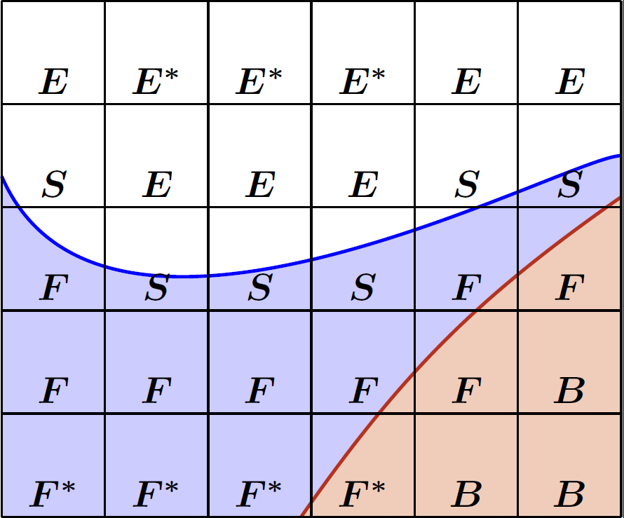
Fig. 2.1 Illustration of the ComFLOW cell labeling system
2.3.2. Discretization and solution method
The Navier-Stokes equations are discretized in time and space. For the time discretization, the Forward Euler method (first-order accurate) or the Adams-Bashforth method (second-order accurate) can be used. The spatial discretization is based on the finite volume method. A choice can be made between (second-order) central discretization and first or second order upwind discretization. For the solution of the discretized Navier-Stokes equations, at each time step a Poisson equation for the pressure, that can be found after rearranging the discretized equations, must be solved. In case of one-phase flow, this Poisson equation can be solved using SOR-iteration with an automatically adjusted relaxation parameter :cite:`botta1985modified`. For most two-phase flow simulations it is advantageous to use the MILU (Matrix Incomplete LU decomposition, see :cite:`botta1999matrix`) or BiCGSTAB pressure solver, as described in section-fixedform-numerical. When the pressure solution is found, the new velocity field is computed and subsequently the free surface is displaced using the VOF-method combined with a local height function :cite:`kleefsman2005water`, :cite:`veldman2007numerical`. Finally, the time step is adjusted using the CFL-condition. The CFL-number is calculated as
where \(u,v,w\) are velocity components and \(h_x,h_y,h_z\) denote
mesh sizes in the corresponding directions.
If the computed CFL-number is greater than cflmax, which is given by the
user in the input file, the time step will be decreased. If the computed CFL-number is
smaller than cflmin during \(10\) successive time steps, the
time step will be doubled.
References