5. Domain and geometry definition
This chapter describes the preprocessing actions for a ComFLOW simulation, including amongst others the geometry definition and the initialization of the flow solution.
The preprocessing program GEODEF has been developed to make it possible to define arbitrary complex geometries for fluid flow simulations. Finite element modeling has many advantages. It is a wide-spread method and there exist many packages that can make finite element descriptions of a geometry that can be as complex as desired.
5.1. Domain definition
The computational domain, in which the simulation is performed, always has a box-like shape, which makes it very easy to define a (semi-)structured grid. The geometry within the domain is defined by means of the preprocessor GEODEF, which produces a file that contains volume and edge apertures for every cell. The volume aperture of a cell defines which part of the cell is open for fluid and which part is closed by the geometry. The edge apertures give similar information for the cell faces. For explanation of the geometry preparation, see Chapter 5.
The domain extents are given by the input parameters xmin, xmax, ymin, ymax, zmin, zmax.
These can be specified in the body of domain/extents/ using the same ordering, for example:
<domain>
    <extents> 0.0 100.0   -10.0 10.0   -30.0 3.0 </extents>
</domain>
results in the computational domain \(\textstyle\{ (x,y,z)\; | \; 0 < x < 100, -10<y<10, -30 < z< 3\}\). The extents should match the boundaries of the computational grid. In 2-D simulations the extents in the third (missing) direction do not affect the simulation results. The extents should always be increasing, hence \(\texttt{xmin} < \texttt{xmax}\) (etc.).
By default the domain boundaries are closed for flow.
This behavior can be modified by changing the body of key geometry/domain_walls/ which must contain
6 flags that indicate if domain walls are open for flow (true) or closed (false).
5.2. Geometry definition
The geometry input for ComFLOW is based on volumetric building blocks (elements). There are two methods available in ComFLOW to calculate the volume and face apertures that correspond with these building blocks.
- The legacy method based on point tests: Each computational cell is covered by a small grid of integration points. Each integration point that is located inside a building block provides a small contribution to the volume aperture.
- An exact method based on exact polyhedral intersections: All intersections between computational cells and the geometric building blocks are calculated. The volume and face apertures are calculated by adding up all contributions.
The method used for the geometry calculations can be selected using the attribute geometry/@method which can be set to either "legacy" or "exact".
The performance and accuracy of the methods are affected by several settings, which include the following:
geometry/@integration_points |
In the legacy approach ( In the exact approach ( |
geometry/@use_aabb_tree |
This attribute can be set to "true" or "false" to enable or disable optimization by means of bounding box trees.
It is recommended to leave this option switched on. |
geometry/@open_up_io_boundaries |
If this attribute is set to "true" boundary conditions are automatically made open for flow using a crude approximation. This is the default behavior.
If set to "false" it is the responsibility of the user to correctly define the geometry at the domain boundaries. This may be useful in special situations, for
example when a ship crosses a domain boundary. |
geometry/@read_apertures |
This attribute can be set to "true" or "false" in order to enable or disable the GEODEF preprocessing step.
If disabled, the geometry is calculated directly by ComFLOW without storage on disk. |
geometry/@apply_cutoff |
Exact method only. This attribute can be set to "true" or "false" in order to enable or disable the cut-off of small volume and face apertures in order to prevent small openings in grid cells which may help to reduce time step restrictions. |
geometry/@maximum_split_level |
Legacy method only. For optimization purposes building blocks are split into smaller tetrahedral building blocks. Splitting is performed until the sizes of the building blocks are similar to the local grid size or the recursion level reaches this number. |
5.2.1. Building blocks
The geometry can be built from the following building blocks:
- 3D: tetrahedron, wedge, brick, ellipsoid, cylinder
- 2D: triangle, quadrilateral, ellipse
These elements should be listed in a file geometry.in.
This file is input for the preprocessor program GEODEF. The
volume and edge apertures (which are the fractions of the ComFLOW cells and
cell faces open to fluid) are output of the preprocessor and input
for ComFLOW. In this chapter the structure of the file
geometry.in will be described and rules that are applied in the
preprocessor are explained. A distinction is made between solid entities
(aperture zero) and empty entities (no solid, aperture one). The empty entities are
open to fluid flow.
For every geometrical entity the following data should be given:
- Type of geometrical entity, which is the first number on the first line. In three dimensions there are five possibilities: tetrahedron, wedge, brick, ellipsoid and cylinder. In two dimensions, three different elements are possible: triangle, quadrilateral and ellipse.
- The second number in the first line is a masking option
exclusive. Ifexclusive=0the building block is used to define a piece of solid geometry (or liquid), whereas , ifexclusive=1the corresponding building block is used to clear a piece of solid geometry (or liquid). NB: When using building blocks with the optionexclusive=1, the final result depends on the order in which the building blocks appear in the input file. appear in the input file. - The third number on the first line is optional and indicates whether the building block is part of a moving object or fixed If the object is moving, this number should be 1. In the case of a fixed object, this number should be 0.
- The following lines specify the coordinates and/or the radii of the element.
The order in which the coordinates of points of the different building blocks are given is very important. For every geometrical building block this will be described directly below.
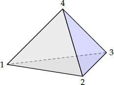
Tetrahedron
The four vertices of the tetrahedron should be given in the following order. Points 1, 2 and 3, given counter-clockwise, form a plane with the normal, pointing inside the tetrahedron, to point 4 (top vertex).
 1 exclusive movingx1 y1 z1x2 y2 z2x3 y3 z3x4 y4 z4
Wedge The six points of the wedge should be given as follows: points 1, 2 and 3, given clockwise, form a plane with the normal, pointing inside the wedge to plane 456. Point 4 should lie opposite point 1, point 5 opposite point 2 and point 6 opposite point 3. To check if a point is inside or outside the wedge, the wedge is divided into 3 tetrahedra. For each tetrahedron it is checked whether the point is inside or outside the tetrahedron. The points in faces 2365, 1364 and 1452 are assumed to be in one plane. If not, the program will calculate the apertures as if the points were in one plane. Then the resulting geometry should be checked carefully.
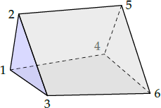 2 exclusive movingx1 y1 z1x2 y2 z2x3 y3 z3x4 y4 z4x5 y5 z5x6 y6 z6
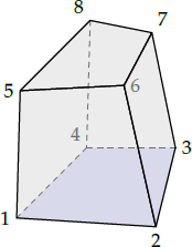
Brick
The brick has eight points. Points 1, 2, 3 and 4, given counter-clockwise, form a plane with the normal, pointing inside the brick to plane 5-6-7-8. Point 5 should be opposite point 1, point 6 opposite point 2, point 7 opposite point 3 and point 8 opposite point 4. To check if a point is inside or outside the brick, the brick is divided into 5 tetrahedra. For each tetrahedron it is checked if the point is inside or outside the tetrahedron. It is assumed that the points in the faces of the brick are in one plane. If not, the program will calculate the apertures as if the points were in one plane. Then the resulting geometry should be checked carefully.
 3 exclusive movingx1 y1 z1x2 y2 z2x3 y3 z3x4 y4 z4x5 y5 z5x6 y6 z6x7 y7 z7x8 y8 z8
Ellipsoid
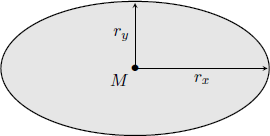
For the ellipsoid, coordinates of the center and radii in X, Y and Z-directions should be given. The main axes of the ellipsoid are restricted to be aligned with the X, Y and Z-axes.
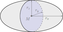 4 exclusive movingxM yM zMrx ry rz
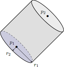
5-6. Circular / elliptic cylinder
The cylinder is defined by the start and end point of the axis and the radius of the base. The axis of the cylinder does not have to be along one of the Cartesian axes.
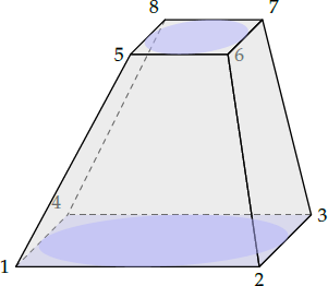
7-8. Quadrilateral / elliptic frustum
The quadrilaterals 1-2-3-4 and 5-6-7-8 must be parallel. For the frustum based on ellipses, the radii are defined by the bounding quadrilaterals 1-2-3-4 and 5-6-7-8, which must be rectangular.
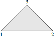
Triangle
The triangle is given by the three vertices. The vertices should be given in counterclockwise order.
 11 exclusive movingx1 y1 z1x2 y2 z2x3 y3 z3
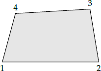
Quadrilateral
The quadrilateral is defined by the four vertices. The vertices should be given in counterclockwise order.
 12 exclusive movingx1 y1 z1x2 y2 z2x3 y3 z3x4 y4 z4
Ellipse
The ellipse should be defined by giving the center and the two radii.
 13 exclusive movingxM yMrx ry
It is absolutely necessary to define the geometrical entities in the above way. Examples of input files and defined geometries are given in Section 5.5.
5.3. Building the geometry (outdated)
5.3.1. Size of the domain and grid.
To build the geometry, for every cell in the ComFLOW domain
the volume and edge apertures should be calculated. Therefore, the
domain and grid distribution should be known in advance. The
preprocessor gets this information from the ComFLOW input
file comflow.in (and optionally from grid.in or grid.cfi, if the grid is
defined outside comflow.in). Every time the grid, domain, geometry or initial liquid configuration changes, GEODEF should be run again.
5.3.2. Initial configuration.
The geometry is built using geometrical entities listed in the
input file geometry.in and the liquid configuration is set up using the
geometrical entities listed in the input file liquid.in. The
starting geometry, before the geometrical entities are put in,
is an empty rectangular domain defined in the file comflow.in.
5.3.3. Processing of the geometry.
After the geometrical entities have been read in, they are processed. The volume
and edge apertures of a ComFLOW cell are calculated using its integration
points (see fixed_form_input/numerical for an explanation of
the number of integration points nrintp). For every integration point in a
cell, its attribute (solid or empty) should be determined. Therefore, for all
the geometrical entities it is checked whether the point is inside or outside the
current entity. If the point is inside the geometrical entity, the
attribute of the point (solid or empty) is determined according to the
attribute of the interior of the geometrical entity. If the point is outside the
geometrical entity, nothing happens.
nrintp: This parameter sets the number of integration points used for the discretization of the geometry. GEODEF checks fornrintppoints per grid cell whether this point is inside or outside the solid geometry, to compute the apertures. As a consequence: param{nrintp}{1} yields a staircase geometry; param[>]{nrintp}{1} gives a more fluent geometry.nrintpis a positive integer. It is advised to use a default value of 3 or 4, higher values may give stability problems in exceptional cases, because of small area apertures. In case of moving bodies, when param{mvbd}{1} the value ofnrintpshould not be taken too small, for sufficient accuracy (say, $geq4$) and should not be taken too large (say $leq 8$) for computational efficiency. However, when param{mvbd}{2} (see cref{section:comflowin:general}) the procedures from geodefare used every time step to compute the apertures of the moving geometry. In that case also larger values can be used and it is advised to takenrintpsufficiently large for accuracy, e.g. param{nrintp}{40}.} In cref{fig:T_geometry} an example of a computational cell with 2 (left) and 4 (right) integration points is given. Cell volume apertures are calculated by counting the number of internal integration points ($bullet$) that are inside the geometry. The cell face apertures are calculated by counting the number of integration points on the cell faces ($times$) that are inside the geometry. The volume aperture ($F^b$) is calculated as the number of points outside the solid geometry, divided by the total number of points: $F^b=frac{3}{4}=0.75$. Following the same procedure on the edges leads to $A^y=0.5$ and $A^x=0$. For the example with 4 integration points the same procedure leads to $F^b=frac{10}{16}=0.625$, $A^y=frac{3}{4}=0.75$ and $A^x=frac{3}{4}=0.75$ which is already significantly more accurate.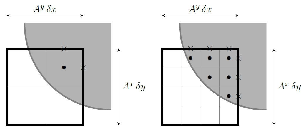
Fig. 5.1 Example of the calculation of geometry apertures using 2 (left) or 4 (right) integration points (gray grids) per grid cell (thick rectangles). The more integration points, the smoother the geometry. The gray area is solid geometry.
The attribute of an integration point
(solid or empty) is determined according to the last element in
which the point lies. So the attribute of a point can change if it is
inside a geometrical entity that is defined later in the geometry.in
input file with a different attribute. In this way, it is
possible to create an object as an union or intersection of
geometrical entities.
For example, if fluid flow inside a sphere is simulated, two elements
should be defined. The first one is a solid brick, which has sizes equal to the
domain given in comflow.in. The second one is
an empty sphere. The first element takes care of the solid outside the
sphere, which is necessary because the starting geometry is an empty
(non-solid) domain (see Section 5.5.2).
5.3.4. Consistent volume and face apertures.
As of ComFLOW v2.3, special care is taken to create consistent volume and face apertures. Moreover, the search algorithm in GEODEF has been improved to prevent the occurrence of faulty ‘virtual walls’. With old versions, in exceptional cases such virtual walls may have been computed. In those cases, the fluid is hampered to move through a ComFLOW cell face, although this face should be fully open for flow. In the left figure an example is depicted of such a virtual wall; the cell face is partly closed.
If a ComFLOW sub-cell is closed (because of a solid body) and its neighbor is open, in principle no flow can move through the face fraction between these two sub-cells. With old versions of GEODEF this may not always have been the case; in such a case the volume and face aperture are not in agreement. In the right figure the depicted volume and face apertures are fully consistent, as computed with the new version of GEODEF.
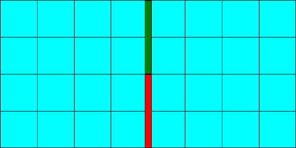
Fig. 5.2 Left: possible virtual walls computed with old versions of GEODEF. Right: consistent volume and face apertures. The blue and dark colors denote ComFLOW sub-cells filled with fluid and solid, respectively. The green and red part of the cell face are open and closed for flow, respectively.
5.3.5. Efficiency of the pre-processor.
Because of computation time, the number of elements should be as small
as possible. The process described above gives a computation time of
GEODEF that is linear in the number of elements, linear in
the number of grid points and cubic in the number of integration
points nrintp (defined in the input file comflow.in). To make
GEODEF more efficient, the apertures of the cells are
initialized first. At this stage, for every computational cell it is
checked whether it is in the neighborhood of a solid element. If
it is not in the neighborhood of a solid element, the volume and edge
apertures are set open for this cell. In that case, it is not
necessary to check all elements for each integration point in this
cell, which makes a large difference in computational time.
5.3.6. Output files.
GEODEF produces two output files that are used by
ComFLOW: apertures.in and geomoving.in.
The file apertures.in contains the volume and edge apertures of every
grid cell. In geomoving.in, for every cell it is determined
whether it is (partly) a fixed geometry, a moving geometry or
completely open for fluid flow.
5.3.7. Calling sequence.
When ComFLOW starts, the file apertures.in is
read, thus it should exist. So the right way to call the programs is:
first GEODEF,
with input files geometry.in and comflow.in
(and optionally grid.in).
Output are the files apertures.in and
geomoving.in.
Finally, call ComFLOW
with a value of 0 for the variable liqcnf in comflow.in
to make sure that liquid_distr.in will be used.
This will start the simulation. In
cref{fig:callingsequence:fixedbodies} this is shown in a graphical way.
5.4. Visualizing the geometry
Sometimes it is useful to have information on the values of the apertures, i.e. the fractions of ComFLOW cells that are open for flow. With the MATLAB GUI it is possible to view the contents of an individual cell by means of the probe function as explained in the manual for the ComFLOW pre- & post-processor.
The files apertures.in and liquid_distr.in are stored in the same format as snapshot files.
Please consult Chapter %s for more information about the file format.
Due to the inclusion of local grid refinement in ComFLOW 4.1.1, the format of the GEODEF output file apertures.in has changed drastically with respect to previous versions.
For now we advise to use the visualization functionality provided in the MATLAB pre- & post-processing tool.
5.5. Examples
In this section several examples will be discussed how to build a geometry
with the pre-processor GEODEF.
As comflow.in and geometry.in are input for
GEODEF, both files are discussed for each case.
Note that only the most important lines of comflow.in are discussed.
A full description of this input file is given in Section 27.
5.5.1. Flow around a solid sphere
The fluid flow around a sphere will be simulated. The
domain is defined in ${INPUT}/comflow.in by means of
------------------------------------------------------------------------
-- domain definition ---------------------------------------------------
xmin   xmax    ymin    ymax    zmin    zmax
-10.0  10.0    -2.0    2.0     -2.0    2.0
------------------------------------------------------------------------
To simulate fluid flow around a sphere located at the origin
\((0.0,0.0,0.0)\)
with radius 1.0, the file geometry.in should
contain the following lines:
4    0    0
0.0  0.0  0.0
1.0  1.0  1.0
Number 4 in the first line means the geometrical entity has shape number 4, which is a sphere. The following 0 means that the sphere is solid. The other 0 means that the sphere is not moving. In the second line coordinates of the sphere centre are given. In the last line radii of the ellipsoid along the X, Y and Z-axes are given. After GEODEF and ComFLOW have been run, the result of the geometry can be shown using Matlab (see Fig. 5.3).
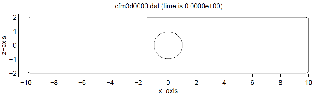
Fig. 5.3 Fluid flow around a solid sphere, cross-section in the XZ-plane.
5.5.2. Flow inside a sphere
To simulate flow inside a sphere with radius 1.0, the domain should be
defined in the file comflow.in as
------------------------------------------------------------------------
-- domain definition ---------------------------------------------------
xmin   xmax    ymin    ymax    zmin    zmax
-1.0   1.0     -1.0    1.0     -1.0    1.0
------------------------------------------------------------------------
The file geometry.in should contain two geometrical entities:
3    0    0
-1.0 -1.0 -1.0
 1.0 -1.0 -1.0
 1.0  1.0 -1.0
-1.0  1.0 -1.0
-1.0 -1.0  1.0
 1.0 -1.0  1.0
 1.0  1.0  1.0
-1.0  1.0  1.0
4    1    0
 0.0  0.0  0.0
 1.0  1.0  1.0
The first geometrical entity has number 3, a brick, and is solid inside. This
brick has exactly the same size as the fluid domain defined in comflow.in.
This geometrical entity is necessary, because without it, the sphere
would be surrounded by empty cells (because of the initial condition
that the domain is empty) and would have empty cells inside. By
defining a solid brick and after that an empty sphere, only flow in
the sphere is possible. The sphere is the second element. It has
element number 4 and is empty inside. The center of the sphere is
point \((0.0,0.0,0.0)\), the radius is 1.0 (so all the three radii must be 1.0).
The resulting geometry is shown in (see Fig. 5.4).
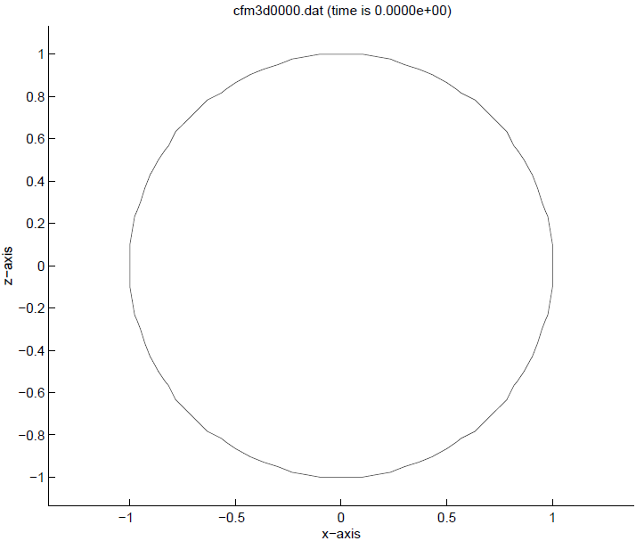
Fig. 5.4 Fluid inside a sphere with radius 1, cross-section in XZ-plane.
5.5.3. Flow around a solid square
In this example, a solid square is built from four smaller squares (as if building a finite element model). The example is displayed in the XZ-plane. The domain is defined as follows:
------------------------------------------------------------------------
-- domain definition ---------------------------------------------------
xmin   xmax    ymin    ymax    zmin    zmax
-10.0  10.0    -2.0    2.0     -2.0    2.0
------------------------------------------------------------------------
The file geometry.in contains descriptions of 4 quadrilaterals:
 12   0   0
-1.0  -1.0
 0.0  -1.0
 0.0   0.0
-1.0   0.0
 12   0   0
 0.0  -1.0
 1.0  -1.0
 1.0   0.0
 0.0   0.0
 12   0   0
-1.0  0.0
 0.0  0.0
 0.0  1.0
-1.0  1.0
 12   0   0
 0.0  0.0
 1.0  0.0
 1.0  1.0
 0.0  1.0
The four quadrilaterals (geometrical entity number 12) are solid. As a union they form a solid square shown in Fig. 5.5.
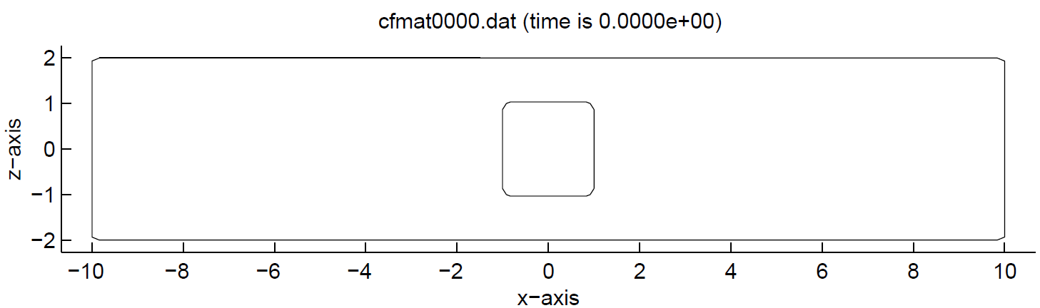
Fig. 5.5 Fluid flow around a solid square in two dimensions.
5.5.4. Flow in and around a rising bubble
In this example, the program GEODEF is used to model a rising
bubble in a water column. The bubble is modeled as a sphere in a 3D
environment, with the following input in comflow.in for the domain definition:
------------------------------------------------------------------------
-- domain definition ---------------------------------------------------
xmin    xmax    ymin    ymax    zmin    zmax
-0.5    0.5     -0.5    0.5     -2.0    1.0
------------------------------------------------------------------------
and the following for the initial liquid configuration:
------------------------------------------------------------------------
-- definition initial liquid configuration -----------------------------
liqcnf lqxmin  lqxmax  lqymin  lqymax  lqzmin  lqzmax
0      -0.5    0.5     -0.5    0.5     -2.0    0.0
------------------------------------------------------------------------
The value of 0 for the variable liqcnf indicates that the
initial liquid configuration is not read from the input line
in comflow.in, but from the separate liquid.in input file.
The file geometry.in is empty in this case.
Note that GEODEF requires
geometry.in as input, so this file should always exist.
The file liquid.in contains two entities:
 3   0
-0.5 -0.5 -2.0
 0.5 -0.5 -2.0
 0.5  0.5 -2.0
-0.5  0.5 -2.0
-0.5 -0.5  0.0
 0.5 -0.5  0.0
 0.5  0.5  0.0
-0.5  0.5  0.0
 4   1
 0.0  0.0 -1.5
 0.25 0.25 0.25
The first ‘liquid’ entity has number 3, a brick, and is filled with
liquid. This brick has the same sizes as the fluid domain defined in
comflow.in, but is less high in Z-direction, indicating a free
surface at \(z = 0.0\). The second entity has number 4, a sphere, and is
filled with the second gas phase. It is important to define the liquid
brick first and after that the empty sphere, because doing it in the other way
would fill the sphere again with liquid. The resulting initial liquid
configuration is shown in Fig. 5.6.
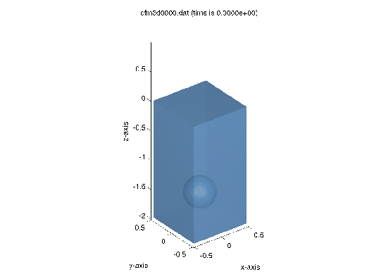
Fig. 5.6 Spherical bubble inside a column of fluid.
5.5.5. Flow in Sloshsat
In this example, the way to build the Sloshsat geometry is
shown. Sloshsat is an experimental satellite, launched to
investigate sloshing liquid in space, and its influence on
overall spacecraft dynamics. Sloshsat can be built as a union of two spheres
with radius 0.228 m and a connecting cylinder with an axis and
radius of 0.228 m. The domain in comflow.in is given by
------------------------------------------------------------------------
-- domain definition ---------------------------------------------------
xmin   xmax    ymin    ymax    zmin    zmax
-0.342 0.342   -0.228  0.228   -0.228  0.228
------------------------------------------------------------------------
In geometry.in, four geometrical entities are defined,
as given below.
The first entity is a brick with size of the domain with solid
inside. The second and third entities are the spheres, the fourth
entity is the cylinder in-between. As the last three entities
have an empty interior, the resulting geometry is a union of these
elements. The geometry is shown in Fig. 5.7.
3  0  0
-0.342   -0.228   -0.228
 0.342   -0.228   -0.228
 0.342    0.228   -0.228
-0.342    0.228   -0.228
-0.342   -0.228    0.228
 0.342   -0.228    0.228
 0.342    0.228    0.228
-0.342    0.228    0.228
4  1  0
-0.114    0.0      0.0
 0.228    0.228    0.228
4  1  0
 0.114    0.0      0.0
 0.228    0.228    0.228
5  1  0
-0.114    0.0      0.0
 0.114    0.0      0.0
 0.228
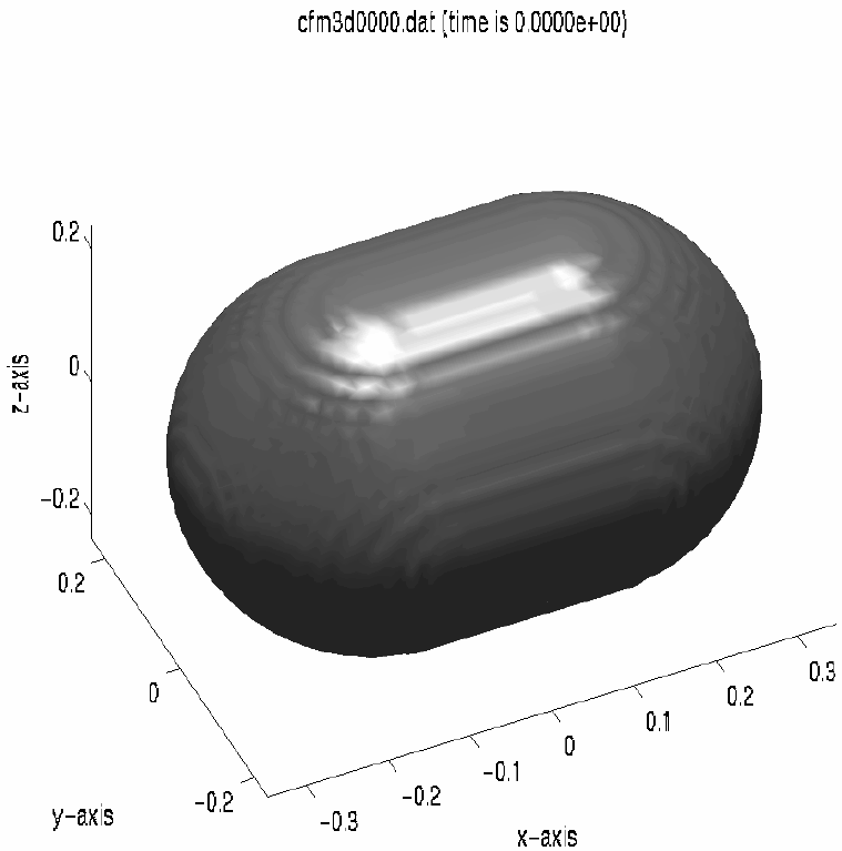
Fig. 5.7 Geometry of sloshsat, 3-D overview picture
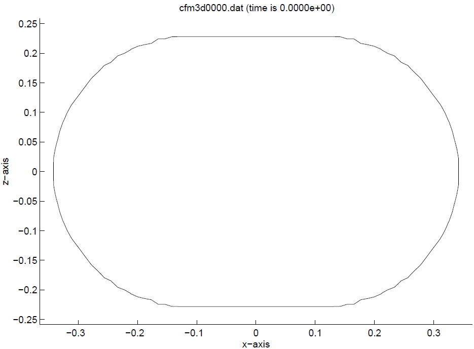
Fig. 5.8 Geometry of sloshsat, cross section in XZ-plane
5.5.6. Coarse finite element model of the bow of a moving ship
In order to give an example of the geometry produced with a finite element modeling package, a very rough finite element model of the bow of a moving ship is built using the finite element package SEPRAN. The number of elements is rather small.
To build this geometry
the following steps are made (see cref{seprancall}). First
the finite element package SEPRAN is used to make a finite element
description of the bow of the ship, as shown in cref{sepran}.
The package
SEPRAN produces an output file
wherein the finite elements are described. A conversion is needed to rewrite
the finite element description to the format of the file geometry.in (this
data format converter is different for each finite element package and should be
written by the user). After the conversion is performed, the
pre-processor GEODEF is invoked to calculate the apertures
needed by ComFLOW.

Fig. 5.9 Calling sequence when the geometry is defined in the finite element package SEPRAN.
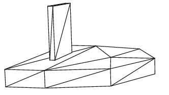
Fig. 5.10 Finite element model of the bow of a ship produced by SEPRAN.
The domain definition in comflow.in is given by:
------------------------------------------------------------------------
-- domain definition ---------------------------------------------------
xmin    xmax    ymin    ymax    zmin    zmax
-40.0   15.0    -30.0   30.0    -6.0    20.0
------------------------------------------------------------------------
The contents of geometry.in is given below.
Out of 27 tetrahedra only the first two entities and last entity are shown.
cref{grofschip} shows the resulting geometry in ComFLOW.
 1   0   1
  -.4000E+02   -.2350E+02   -.6000E+01
  -.4000E+02    .2350E+02    .0000E+00
  -.4000E+02   -.2350E+02    .0000E+00
  -.2600E+02    .2350E+02    .0000E+00
 1   0   1
  -.4000E+02   -.2350E+02   -.6000E+01
  -.4000E+02    .2350E+02   -.6000E+01
  -.4000E+02    .2350E+02    .0000E+00
  -.2600E+02    .2350E+02    .0000E+00
...
....24 other tetrahedra....
...
 1   0   1
  -.3200E+02   -.7500E+01    .0000E+00
  -.3200E+02   -.7500E+01    .2000E+02
  -.3000E+02   -.7500E+01    .2000E+02
  -.3000E+02    .7500E+01    .2000E+02
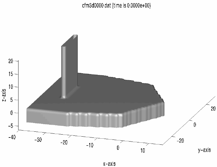
Fig. 5.11 The geometry of the bow of a ship in ComFLOW.