11. Boundary conditions
11.1. Domain boundary conditions
At the boundaries of the domain inflow- and outflow conditions can be specified.
Domain boundary conditions are described in the XML key(s) /comflow/boundaries/boundary[*].
The following basic example defines generating and absorbing boundary conditions (see Section 11.1.4) on all sides of the domain:
<boundaries>
    <boundary io="11">   0.   0. -Inf Inf  -Inf Inf </boundary>
    <boundary io="11"> 100. 100. -Inf Inf  -Inf Inf </boundary>
    <boundary io="11"> -Inf Inf    0.   0. -Inf Inf </boundary>
    <boundary io="11"> -Inf Inf  100. 100. -Inf Inf </boundary>
<boundaries>
On parts of the domain boundaries where the input file does not define any condition, the implementation default to a no-slip condition. Details on how to apply partial-slip conditions are described in Section 11.2.
The attribute boundary[*]/@io selects the type of boundary condition to be used.
The body of the key boundary[*]/ defines the plane (section) on which the boundary condition is applied in the following order: xmin, xmax, ymin, ymax, zmin, zmax.
Boundary conditions are often applied on the entire domain boundary, which can be realized by using extents of -Inf to +Inf.
In order to determine the orientation of the boundary plane, at least one coordinate extent has to be empty, so xmin=xmax, ymin=ymax or zmin=zmax.
More details for the various types are described in the following sections.
11.1.1. Basic wave inflow condition (1)
This boundary condition imposes incoming flow (waves) by means of a Dirichlet condition for the velocity and the water level. In many situations this boundary condition performs well enough, however, for reduced reflections it may be interesting to consider the generating absorbing boundary condition as described in Section 11.1.4.
11.1.2. Neumann outflow condition (2)
When the attribute boundary[*]/@io is set to 2 the velocity, pressure and water height in the exterior of the domain
are approximated using constant extrapolation.
This is a very simple boundary condition and does not perform very well in wave simulations.
Often, better performance may be obtained by using the more advanced generating and
absorbing boundary condition (GABC) which is described in Section 11.1.4.
11.1.3. Sommerfeld outflow condition (4)
Note
This boundary condition has become obsolete. It is strongly recommended to use the new-style absorbing boundary condition, which can also be tuned to match a single regular wave component, see Section 11.1.4.
It is also possible to apply a Sommerfeld outflow condition by setting boundary[*]/@io="4".
The Sommerfeld condition only performs well for regular waves that are not too much disturbed by an object.
Typically lower reflection rates can be obtained with the new-style (G)ABC boundary condition or by applying a damping zone.
The Sommerfeld boundary condition uses a wave velocity, which is computed from the wave period and wave number. The latter is based on the dispersion relation and hence also depends on the water depth. The wave velocity follows from the wave period and water depth as specified in the wave modeling section of the input file (see Chapter 10).
11.1.4. Generating and absorbing boundary condition (11)
At a wave inflow boundary the velocity and water height are prescribed according to the selected wave model (see cref{section:comflowin:waves}). As an alternative, it is possible to use a non-reflective generating boundary condition (GABC) by setting param{io}{11}. The parameters for the absorbing boundary condition are described in cref{section:comflowin:gabc}. Note that generating boundary conditions can only be applied on the {it left} sides of the domain.
Compared with the Sommerfeld boundary condition, the wave velocity at the outflow boundary is no longer prescribed, but determined from the velocity and pressure field.
Please note the following limitations:
- The (G)ABC boundary condition can not be applied in combination with two-phase flow.
- The boundary plane on which the (G)ABC is applied has to be entirely open for flow starting at the bottom of the domain (\(z=\texttt{zmin}\)).
- If the wave propagates parallel to the X-direction, under zero angle of incidence (param{beta}{0}), the boundaries in the XZ-plane (param{plane}{2}) can not be specified as GABC boundaries.
- Similarly, if the wave propagates parallel to Y-direction under an angle of incidence param{beta}{90}, the boundaries in the YZ-plane (param{plane}{1}) can not be specified as GABC boundaries.
- The (G)ABC can also be applied in “non-wave” simulations (i.e. when param{wave}{0}).
In that case make sure to specify a reasonable water depth in the wave input section (see cref{section:comflowin:waves}).
Typically this comes down to setting
waterdequal to -zmin.
In order to prevent wave reflection from the domain boundaries, a generating (and) absorbing boundary condition (GABC) has been implemented. The GABC can be used at the inflow ends of the domain, where waves are generated (incoming waves), and it can be used at the outflow ends of the domain, where waves leave the domain (outgoing waves). % , as long as the wave is propagating % with an angle of incidence of $0!<!$ {tt beta} $!<!90$. % In case of parallel propagation, the GABC can not be specified on the side walls that % are parallel to the propagation direction of the waves.
To define a GABC inflow or outflow, first define the
in- and outflow coordinates and give io
the value 11, as explained in cref{section:comflowin:inoutflow}.
Subsequently, give the following variables appropriate values:
------------------------------------------------------------------------
-- absorbing boundary condition ----------------------------------------
bcl* bcr*  gabc  a0    a1    b1    kh1     kh2~   alfa1  alfa2~
1    1     1     1.05  0.12  0.31  1.345   5.0    0.0    0.0
------------------------------------------------------------------------
The coefficients
bclandbcrare not used and must be set to 1.The parameter
gabcdetermines the order of the absorbing boundary condition. If a minus sign is added the wave number of the outgoing wave is not determined from the local flow solution but is taken equal to that of the incoming wave as specified in the ComFLOW input file. Depending on the value ofgabcadditional parameters need to specified:\ begin{center} begin{tabular}{>{bf}ccccccccc} rowcolor{gray!40} lstinline|gabc| & bf varname{a0} & bf varname{ a1} & bf varname{ b1} & bf varname{ kh1} & bf varname{ kh2} & bf varname{ alfa1} & bf varname{ alfa2} &\ 1 & x & x & x & x & - & - & - & (ir)regular waves\ 2 & x & x & x & x & x& x& x & (ir)regular waves\ -1 &- & - & - & - & - & - & - & regular waves\ -2 &- & - & - & - & - & - & - & regular waves end{tabular} end{center} When param{gabc}{1} is chosen, the traditional first-order GABC will be applied at the corresponding boundaries. In this case, onlya0,a1,b1,kh1andalfa1need to be specified in this section andkh2,alfa2are ignored.When param{gabc}{2} is chosen, the second-order GABC will be applied, which has superior performance especially in terms of directional effects. In this case,
a0,a1,b1,kh1,alfa1andalfa2need to be specified in this section.Note
When a minus sign is added to the parameter
gabc, the (G)ABC-1 (param{gabc}{-1}) or ABC-2 (param{gabc}{-2}) boundary condition is automatically tuned for the regular wave as defined in the wave input section (see cref{section:comflowin:waves}). In this case the input for the remaining coefficientsa0,a1,b1,kh1,kh2,alfa1,alfa2is ignored.This option replaces the old-style Sommerfeld boundary condition (param{io}{4}).
The coefficients
a0,a1andb1originate from the approximation of the linear dispersion relation:\[c_a = \sqrt{{g}{h}}\frac{a_0 + {a_1}{({k}{h})^2}}{1 + {b_1}{(kh)^2}}\]With the current chosen values of
a0,a1andb1, the dispersion relation is approximated as shown in cref{pade_approximation}. Note that \(k\) is the wave number which is determined from the local flow solution and \(h\) is the water depthwaterdwhich is specified in the input file (see cref{section:comflowin:waves}).a0,a1andb1can be changed to accurately approximate a different part of the dispersion relation. Not every set of coefficients is stable, but if the following requirements are satisfied, stability is guaranteed:\[\begin{split}\frac{a_0}{\pi^2}< a_1 < \frac{4a_0}{\pi^2} \\ a_1 < b_1 < \frac{4}{\pi^2} \label{eq:ineqa1}\end{split}\]Always remember that the intention is to approximate the true dispersion relation as good as possible. A better approximation yields less reflection. For regular waves of which the properties are known on forehand it is possible to make the approximation exact. To do so, set
gabcto -1 or -2 and specify the incoming wave as explained in cref{section:comflowin:waves}.For regular waves,
kh1can be set to the $kh$-value of the regular wave. For the irregular waves, the value forkh1needs to be set to the kh-value associated with the peak of the input spectrum. When, for instance, the input spectrum contains wave components over a range from kh = 0 to kh = 5, thenkh1should to be set to 2.5.For both regular and irregular waves, a default value for
kh2will be provided upon the completion of the tests.alfa1determines the angle in degrees for which the GABC provides the best absorption. For regular waves, this value can be set to the angle of incidencebetadefined in cref{section:comflowin:waves}. For irregular waves, ``alfa1} can be set to the main propagation direction of the wave.For both regular and irregular waves, a default value for
alfa2will be provided upon the completion of the tests.
The GABC can be defined in both YZ-planes and XZ-planes.
The performance for waves under an angle the non-reflective properties depend on
the chosen settings for alfa1 (alfa2).
Waves that travel parallel to the (G)ABC boundary plane remain unaffected:
for those waves effectively a free-slip boundary condition is applied.
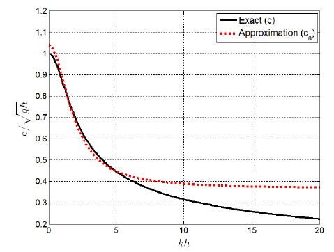
Fig. 11.1 Approximation of the linear dispersion relation using the following set of coefficients: a0 =1.05, a1 =0.12 and b1 =0.31.
Together with all other ComFLOW material,
an auxiliary MATLAB script is provided,
viz. coefficient_optimization.m,
which can be used to compute the coefficients a0, a1 and b1
that are optimal for a specified range of kh values.
The value of kh for comflow.in still corresponds to the peak
of the input spectrum.
Note that this script was originally designed for the traditional first-order GABC boundary condition.
Finally, note that the (G)ABC boundary condition modifies the matrix structure which cannot be handled by all matrix solvers.
Make sure to use param{solver}{5} (see fixed_form_input/numerical).
When using this solver, also make sure to optimize its efficiency by adjusting the parameter droptolbc following the instructions in the same section.
11.1.5. Free-slip condition (28)
At free-slip boundaries (param{io}{28}) the tangential velocities in the exterior are set equal to those in the interior such that viscous stresses become equal to zero. The liquid distribution is assumed to be uniform across the boundary. Internally this boundary condition is simply replaced by boundary type 101 (see below) with the normal component of the velocity set to zero and the tangential components obtained by extrapolation from the interior.
11.1.6. Atmospheric condition (31)
This boundary condition can be used in two-phase simulations to fix the atmospheric pressure and impose velocities (“wind speeds”) at the top boundary of the domain. The atmospheric boundary condition, to be defined at the top of the domain, can be used for two-phase simulations of waves. The main purpose of this boundary condition is to fix the pressure level, which may drift away during two-phase simulations in open domains. At the atmospheric boundary, the pressure is always zero (neutral atmospheric value) and the vertical velocity component \(w\!=\!0\). Moreover, the horizontal velocity component \(u\) is prescribed, which represents the windspeed of the undisturbed atmosphere above the water. This windspeed is also prescribed at the inflow boundary, above the incoming wave. An example is as follows
------------------------------------------------------------------------
-- definition of in- and outflow boundaries ----------------------------
nrio
3
io   plane xmin   xmax     ymin  ymax   zmin   zmax
1    1     0.00   0.00    -0.50  0.50  -10.00 14.00
4    1     100.00 100.00  -0.50  0.50  -10.00 14.00
31   3     0.00   100.00  -0.50  0.50   14.00 14.00  1.23  0.0  0.0
------------------------------------------------------------------------
In the example,
at \(x\!=\!0\) an inflow boundary is defined (incoming wave) and at \(x\!=\!100\) a Sommerfeld
outflow boundary is specified.
The atmospheric condition (param{io}{31}) is put at height \(z\!=\!14.0\), which is the top of the domain zmax.
The windspeed is \(u\!=\!1.23\), directly from \(t\!=\!0\), as both iostart and iofull are 0.0.
During the simulation,
the windspeed is imposed at the top of the domain and above the incoming water wave.
The air inside the domain (above the water) also gets the same (initial) windspeed at \(t\!=\!0\).
To prevent from undesirable initial effects, it is recommended to start with a wave at rest (param{wvstart}{0},
param{ramp}{1}), see cref{section:comflowin:waves}.
11.1.7. Basic Dirichlet and Neumann conditions (101, 102, 104)
Furthermore, the following velocity/pressure boundary conditions can be used. When the velocity is specified, a Neumann condition for the pressure is applied. When the pressure is specified, it is combined with a Neumann condition for the velocity. The flow is assumed to be perpendicular to the domain, i.e. external tangential velocities are set to zero.
begin{center} begin{tabular}{p{.1linewidth}p{.7linewidth}} arrayrulecolor{white} rowcolor{gray!10} 101 & boundary flow velocity specified ($u=u_{spec}$)\ hlinehline rowcolor{gray!10} 102 & outside pressure specified ($p=p_{spec}$)\ hlinehline
rowcolor{gray!10} 104 & hydrostatic pressure based on the actual water level plus an outside pressure (\(p=p_{hydr}+p_{in}\))
end{tabular} end{center}
The following additional parameters have to be specified for these boundary conditions:
iospec: prescribed velocity or pressure valueiostart,iofull: the prescribed velocity/pressure value increases linearly from 0.0 toiospecbetween timesiostartandiofull. After timeiofull, the prescribed value is constant. Note that in case of linearly increasing velocity, atiofullthe boundary condition suddenly switches from (prescribed) constant acceleration to zero acceleration.opt: Undocumented option.
11.1.8. Flux matching condition (103)
At flux matching boundaries the velocity is determined by calculating the total discharge through all other open boundaries and dividing it by the size of the specified boundary section.
11.1.9. Obsoleted boundary conditions (111,112,113,114)
These boundary conditions have become redundant and are only supported for backwards compatibility. Their implementation is identical to that of conditions 101,102,103,104 respectively.
11.1.10. Geometry definition near domain boundaries
By default the exterior of the domain is assumed to be solid, hence not open for flow. When an inflow- or outflow boundary is specified, as described in cref{section:comflowin:inoutflow}, the geometry is extrapolated from the interior to the exterior.
It is possible to overrule the standard behavior of a closed exterior by setting the parameter bndspec to 1 and specifying the options xlopen, xropen, etc. (see cref{section:comflowin:domain}).
If bndspec is set to 1, GEODEF also generates geometry information in the exterior of the domain and ComFLOW makes no modifications at in- and outflow boundaries afterwards.
11.2. Domain extensions
11.2.1. Symmetry planes
Symmetry planes are special boundary conditions that can only be applied to an entire domain boundary. The geometry and all flow variables are mirrored over the symmetry plane, while the normal velocities on the plane are zero. For moving body cases, it is possible to let the symmetry plane intersect the moving body. In that case only half of the body is considered and forces perpendicular to the symmetry plane are set to zero. The center of mass must be located on the symmetry plane.
Symmetry planes are set in the key domain/symmetry/ which contains 6 flags that can be set to true or false
for the “X-left”, “X-right”, “Y-left”, “Y-right”, “Z-left” and “Z-right” boundaries of the domain, respectively.
The full simulation domain can be reconstructed afterwards by means of the ComFLOW post-processing utilities in MATLAB.
11.2.2. Periodic boundaries
Periodic extension of the computational domain can be enabled or disabled in the body of the key domain/periodic/ which contains 3 flags that can be set to true or false
for the X-, Y- and Z-direction, respectively.
11.3. Definition of a numerical beach
In order to prevent reflections of waves from the outflow boundary into the interior of the domain, an option for a so-called ‘numerical beach’ has been implemented. The beach is usually one or two wavelengths long, with a damping function to be determined depending on the wave frequency. The wave is damped by adding a pressure term at the free surface that counteracts the wave motion.
This pressure term depends on the wave period, amplitude and wave number. The latter is based on the dispersion relation and hence also depends on the water depth. In case of a complex wave consisting of multiple wave components (wave=4), user defined waves (wave=51) or absence of waves (wave=0), wave quantities specified incomflow.in(seefixed_form_input/waves) are used to compute the pressure term. A numerical beach is not possible in case of a greenwater simulation (seefixed_form_input/greenwater).
------------------------------------------------------------------------
-- definition of numerical beach in positive x-direction ---------------
numbch  dampto* slope   bstart
1       0       0.03    651.0
------------------------------------------------------------------------
When numbch equals 0, no damping zone will be used. When the parameter numbch equals 1,
a part of the domain in the
positive X-direction becomes a damping zone. When a damping zone is present, the
wave will always be damped completely, which is shown by the zero
value of parameter dampto* (which is currently the only valid value).
The slope and length of the beach can be chosen using cref{dampingzone}. For regular waves, the following steps have to be taken.
- Choose the amount of reflection ($r_{tot}$) that should be permitted. This amount of reflection is calculated theoretically, and is only valid for a perfectly regular wave.
- Calculate the frequency of the regular wave (in rad/s). The frequency is placed at the horizontal axis.
- Determine the length of the numerical beach using the curved lines. At the left coordinate axis, the accompanying values are placed.
- Determine the slope of the numerical beach, using the straight lines with the values of the right coordinate axis.
The choice of the level of reflection should be made pragmatic. For example, when a wave is simulated with frequency of
0.5 rad/s, the choice for \(r_{tot}=0.01\) cannot be made, because the
number of wavelengths needed for the damping zone exceeds 5. So, a better choice would be
\(r_{tot}=0.05\), which means that theoretically 5% of the wave will be
reflected. In that case, the length of the beach should be
approximately one wavelength, and the slope equals 0.09 (which can be
read from the figure). Then, in the input file,
the parameter slope will be given the value 0.09.
The parameter bstart, which gives the point on the X-axis where the beach starts, should
be one wavelength before the end of the domain (see also the case WaveLoadingSPAR included in the examples directory).
- begin{figure}[htb]
- begin{center}
- resizebox{13cm}{!} {includegraphics{figs_manual/dampfig}}
end{center} caption[Combination of required length and slope of the dissipation zone.] {Combination of required length and slope of the dissipation zone (numerical beach).} label{dampingzone}
end{figure}
When simulating steeper waves using 2nd- or 5th-order Stokes wave theory, the water level in the domain rises, because more water flows in than out. This can be prevented by defining an outflow boundary at the boundary opposite to the inflow boundary, where hydrostatic pressure is prescribed. This is recommended and can simply be done by adding an outflow boundary at $x$=``xmax`` in the previous section.
11.4. Partial-slip condition
The default boundary condition for solid walls is no slip. Instead of no-slip, the boundary conditions for solid walls can be changed to free slip or partial slip. Please note that the partial-slip settings affect all solid boundaries of both static and moving objects.
-------------------------------------------------------------------------
-- partial slip----------------------------------------------------------
pscnf   psl     fsxl~   fsxr~   fsyl~   fsyr~   fszl~   fszr~
0       0.0     0       0       0       0       0       0
-------------------------------------------------------------------------
pscnfcontrols whether partial slip is switched off (param{pscnf}{0}) or partial slip is applied (param{pscnf}{1}). The default value is param{pscnf}{0}, which gives no-slip boundary conditions at solid walls everywhere.pslcontrols the level of partial slip: param{psl}{0.0} gives a no-slip condition, whereas param{psl}{‘inf’} approximates the full free-slip condition. Any positive real value is possible.fslinext: This parameter controls the velocity extrapolation near the free surface. If param{fslinext}{0}, robust zero-th order (constant) extrapolation is applied everywhere. If param{fslinext}{1}, first order (linear) extrapolation is used when possible. If insufficient information is available (e.g. near solid objects) the method automatically switches back to the more stable constant extrapolation.